Restaurant Sales Forecasting: How to Predict Demand and Plan Inventory

Most multi-location restaurant groups are forecasting. Almost none are doing it in a way that actually changes what they order.

The operators who consistently hold food cost below 30% share one habit: they treat sales forecasting not as a finance exercise, but as a purchasing system. The forecast is not a number the GM reviews on a Monday morning. It is the mechanism that determines exactly how much protein gets ordered on Wednesday, which supplier gets called first, and how much buffer stock to hold at each location.

Food cost runs between 25 and 35% of revenue for most restaurant operations. A 2 to 3 percentage point improvement is not a rounding error — across operators on the Supy platform, it is regularly the difference between a profitable quarter and a loss-making one. Sales forecasting, done properly, is what closes that gap.

This guide covers the five operational steps to build a sales forecasting process that connects directly to procurement. By the end, you will know exactly what data you need, how to translate cover counts into ingredient-level demand, how to calculate safety margins by ingredient category, and what accuracy target to aim for at your current stage of growth.

Step 1: Gather and Clean Your Historical Sales Data

A forecast is only as reliable as the data behind it. The single most common reason restaurant forecasts fail is not a bad model — it is incomplete or uncleaned historical data fed into an otherwise reasonable process.

You need a minimum of 12 months of daily item-level sales data before you can build a forecast worth trusting. Restaurant demand has strong seasonal cycles: Christmas and festive trading peaks, summer tourist seasons, the August bank holiday surge, major sporting events. A 6-month dataset misses at least one of these cycles entirely. A 12-month dataset captures a full rotation and lets your model learn the pattern before making predictions.

Beyond duration, the structure of the data matters as much as the length. Revenue totals are not enough.

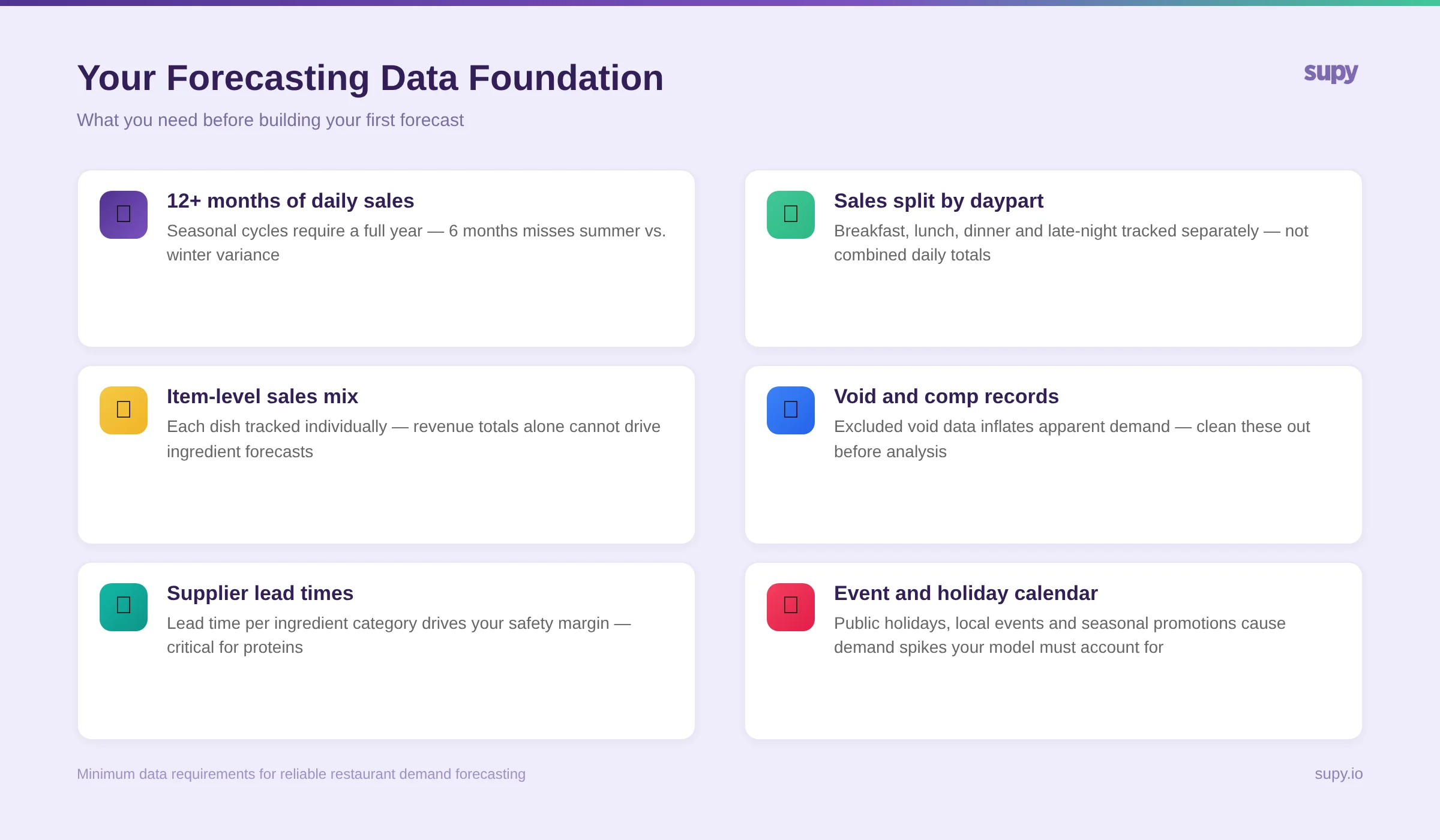
A note on data quality that most operators miss: your POS records two types of zero-revenue transactions that need to be treated differently. Voided orders — cancelled before any food is prepared — should be excluded from your ingredient demand figures because no ingredients were consumed. Comped orders — prepared and served without charge — should stay in your data, because the kitchen still used the ingredients. If you strip comps out of your demand figures, you will systematically under-order for the volume you are actually serving.

For operators running multiple locations, the data consolidation step is often where forecasting stalls. Across the mid-scale groups we work with — typically 5 to 20 sites — the most common bottleneck is not the forecast methodology but the data estate underneath it: four POS systems, three export formats, two different ways of categorising the same menu item across sites. This is a systems problem worth solving before investing in forecasting methodology. A fragmented data estate makes accurate multi-site forecasting structurally impossible, regardless of how good your algorithm is.

Step 2: Choose the Right Forecasting Method for Your Operation

There is no single forecasting method that works for all restaurant operations. The right approach depends on your scale, your data maturity, and the time your team can realistically invest in the process each week.

The most useful framework is to think in three tiers, based on operational complexity rather than ambition.

Before going into each tier: MAPE (Mean Absolute Percentage Error) is the standard measure for demand forecasting accuracy. A 10% MAPE means your forecasts are off by an average of 10% against actual demand. Lower is better. The gap between a manual process and a connected AI system is typically 8 to 12 percentage points of MAPE — which translates directly to 8 to 12 percentage points less over-ordering and waste.

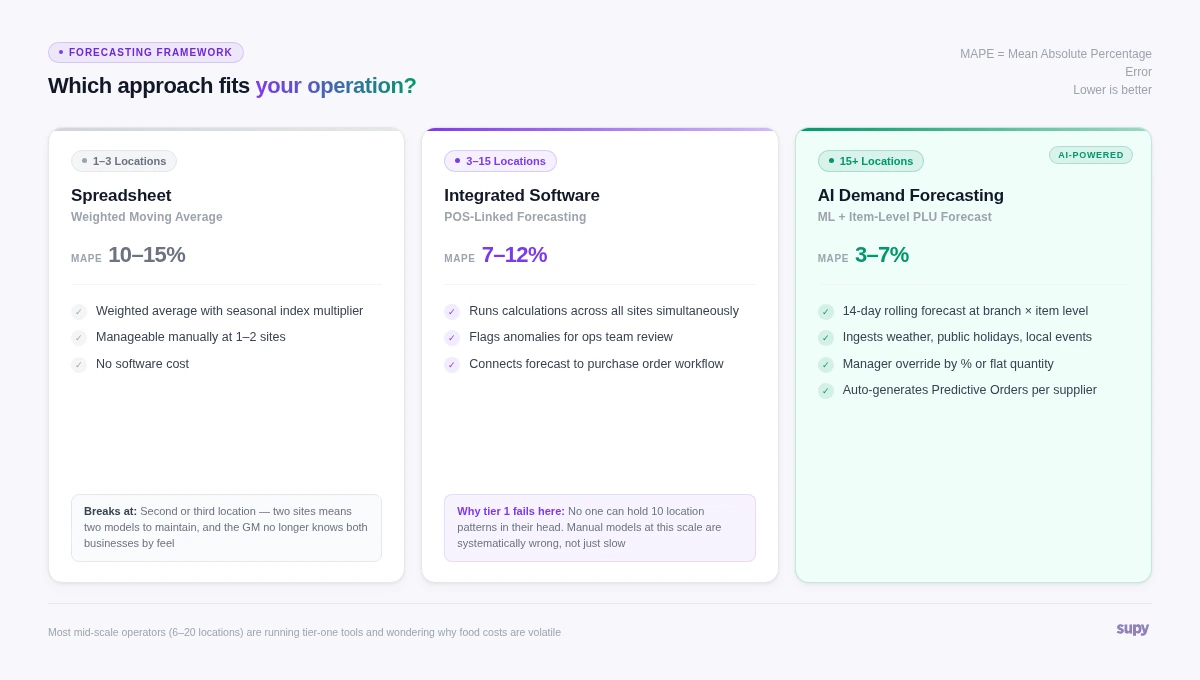
At 1 to 3 locations, a well-maintained spreadsheet running a weighted moving average can get you to 10 to 15% MAPE. Weight recent weeks more heavily than older data. A simple formula: assign 40% weighting to the most recent four weeks, 35% to weeks 5 to 8, and 25% to weeks 9 to 12. Apply a seasonal index on top by comparing the same week from the previous year as a multiplier. This is manageable manually and produces material improvements over pure gut feel. The approach works until it doesn't — which typically happens the moment you open a second location and realise you are now maintaining two separate models while also running operations.

At 3 to 15 locations, the manual approach breaks down — not because the maths gets harder, but because the data volume and the number of variables makes it impossible to maintain without someone doing it full-time. No GM can hold 12 site-level trading patterns in their head simultaneously, each with slightly different menu mix, different local event calendars, different supplier lead times. At this scale, you need POS-integrated forecasting software that runs calculations across all sites simultaneously and flags anomalies for your operations team to review.

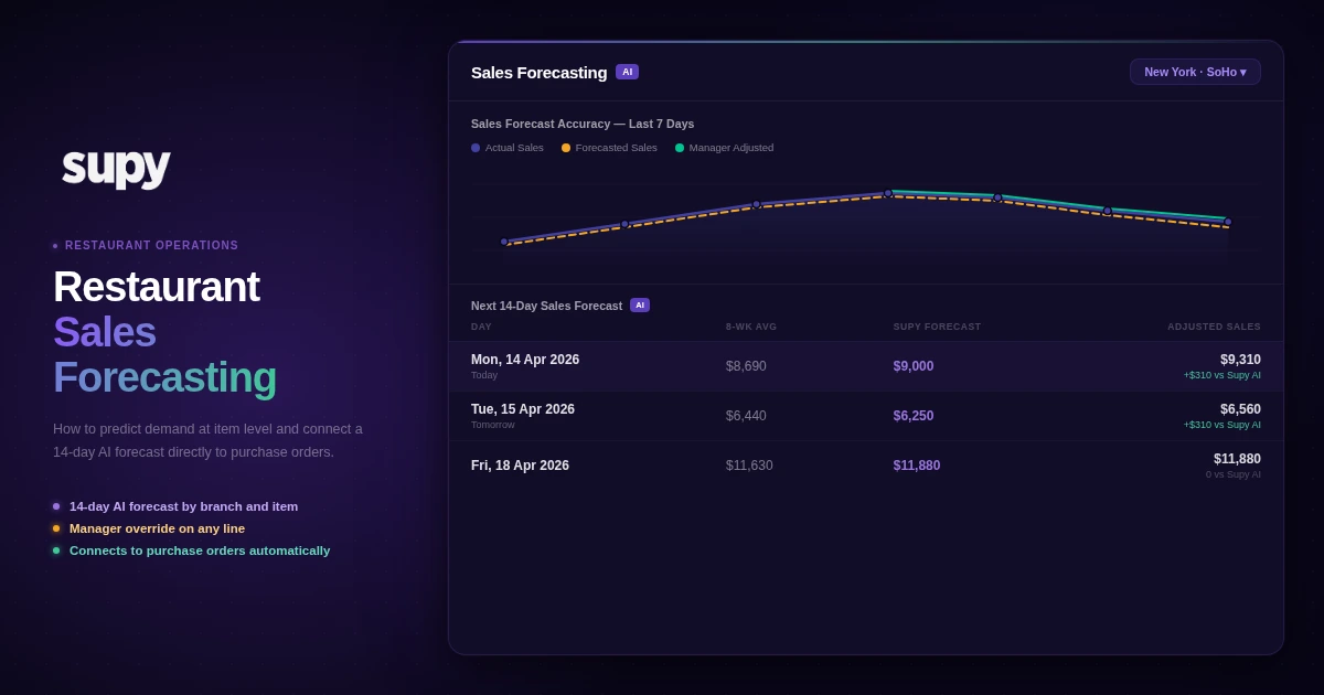
At 15 or more locations, machine learning-based demand forecasting pays for itself clearly. Supy's forecasting engine produces a 14-day rolling branch-level forecast, updated every day as new POS data arrives. It does not just forecast total daily revenue — it forecasts at item level, using your full PLU catalogue. "Tuesday at Manchester Piccadilly: 68 Classic Burgers, 42 Caesar Salads, 23 Sea Bass portions." Managers can then adjust the total day forecast by a flat amount or percentage if they have specific intelligence — a private event, a road closure, an unseasonably warm day — or adjust individual item quantities where they know something the model does not. The accuracy improvement over manual processes — typically from 10 to 15% MAPE down to 3 to 7% — compounds directly into food cost reduction. The longer the system runs, the more accurate it becomes, learning your location-specific patterns and seasonal cycles from the full historical record rather than just a rolling window.

The honest question is not "should I be forecasting?" but "are my forecasting tools matched to the scale I am actually operating at?" Most mid-scale operators are running tier-one tools and wondering why their food costs are volatile.

Step 3: Translate Covers into Ingredient-Level Demand

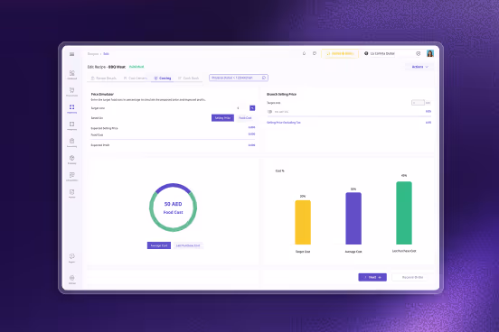
A cover forecast tells you how many guests to expect. A purchasing decision requires something more specific: how many kilograms of chicken thigh, how many litres of cream, how many portions of parmesan. The bridge between those two things is your recipe library — and getting this step right is where forecasting starts to deliver actual purchasing value.

The calculation requires three inputs for each menu item: the forecasted cover count for that item, the portion weight in the recipe card, and the yield factor for each primary ingredient.

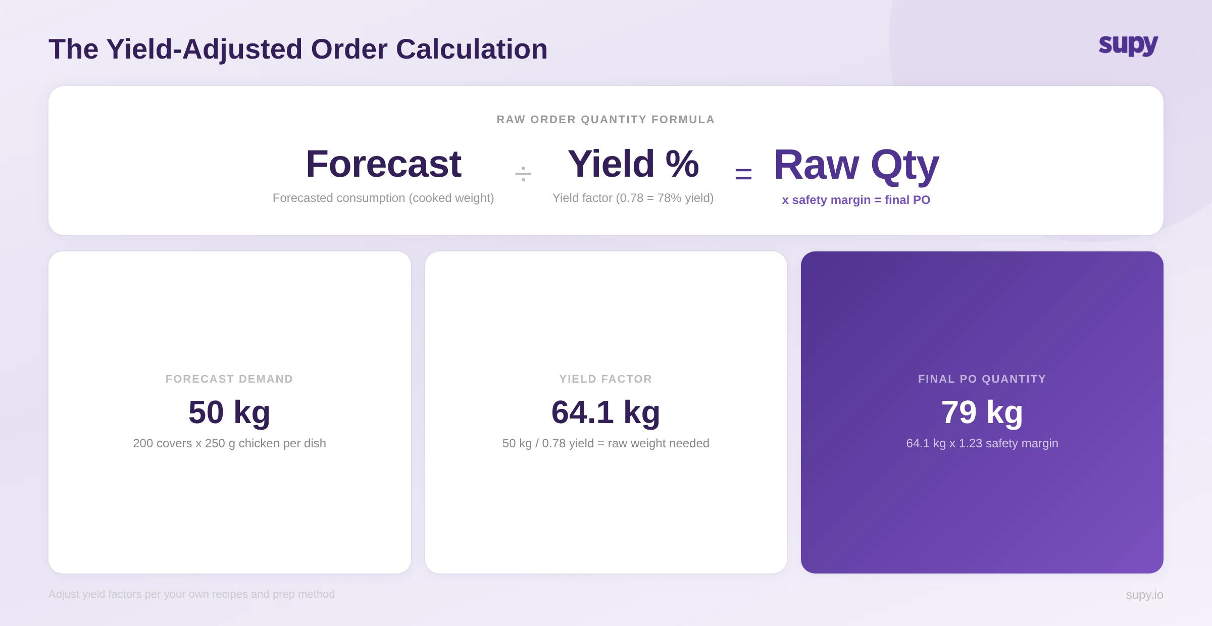
The yield factor is the variable most operators either estimate badly or ignore entirely. Here is what that costs.

At Marina Grill, a casual dining group with seven locations, the kitchen team was building purchase orders based on a 90g per portion figure for chicken thigh — the recipe card weight. What they had not accounted for was yield: actual prep and cooking loss brought their raw-to-plated ratio to 0.78, meaning only 78% of raw chicken weight survived the full process. The correct raw order quantity per portion was not 90g but 115g.

Applied across their highest-volume protein at seven sites, they had been under-ordering chicken by 28% for six months. The consequence was not waste — it was the opposite. They were consistently running short mid-service, covering the gap with last-minute supplier calls at spot prices, watching their chicken cost percentage climb without being able to identify why. The issue was not the supplier. It was a number in a recipe card.

Applying yield factors correctly and consistently across your full recipe library changes the character of your purchasing from reactive to planned. The difference in protein order accuracy alone is typically 15 to 25% when switching from raw recipe weights to yield-adjusted quantities.

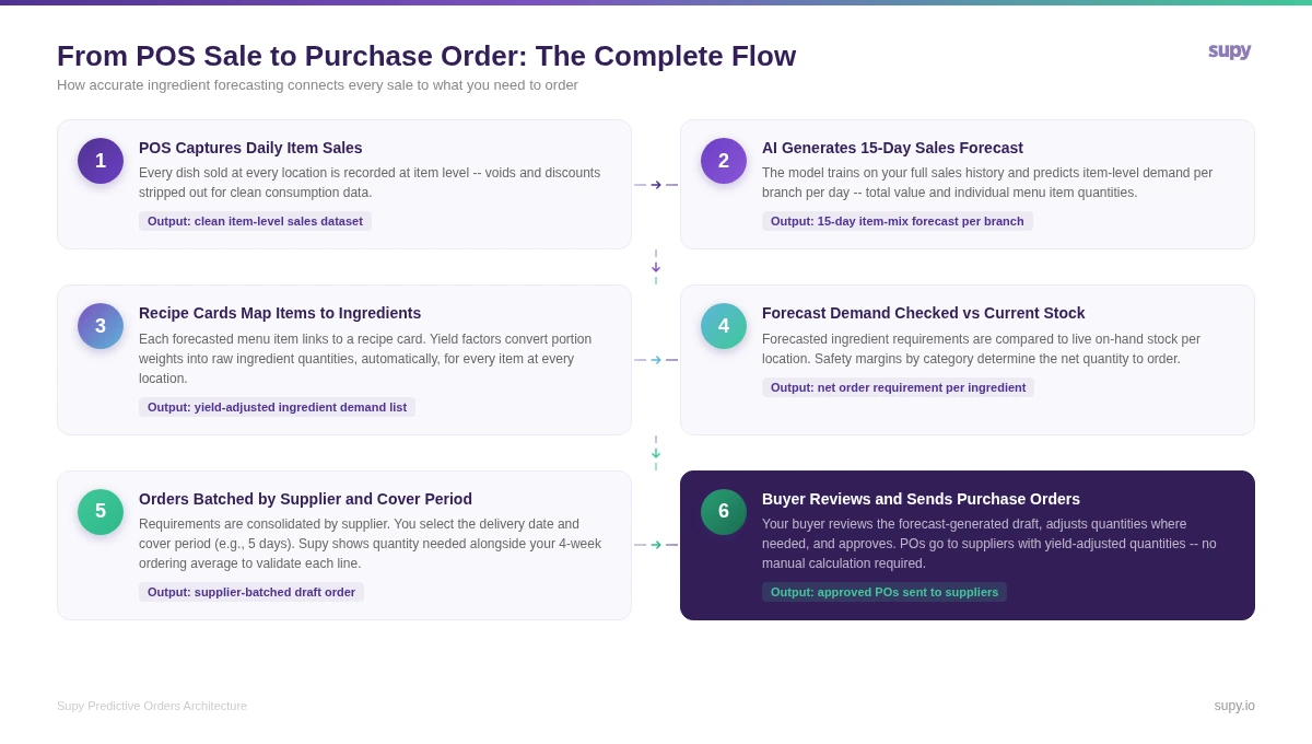
In Supy, each recipe card stores yield factors per ingredient. Because the platform forecasts at item level — knowing how many units of each menu item will be sold at each location, not just total revenue — it applies your recipe cards directly to the forecast output. For every forecasted item, the system looks up the recipe, applies the yield factor to each ingredient, and calculates the raw quantity required. The output is a complete ingredient demand list per supplier, per location, per day — produced automatically, without your procurement team handling a single calculation.

Step 4: Account for Variability and Build Location-Specific Safety Margins

A yield-adjusted quantity calculation tells you what you need in a perfectly predictable world.

Restaurants are not a perfectly predictable world. A safety margin is the buffer between what the model says and what you actually need to hold — and it needs to be calibrated by ingredient category, not applied as a flat percentage across everything.

The framework for calculating a safety margin requires two inputs: demand variance (the standard deviation of forecast error for that category) and lead time variance (the standard deviation of your supplier's delivery reliability). Together they determine the statistical buffer needed to avoid running out of stock before your next delivery.

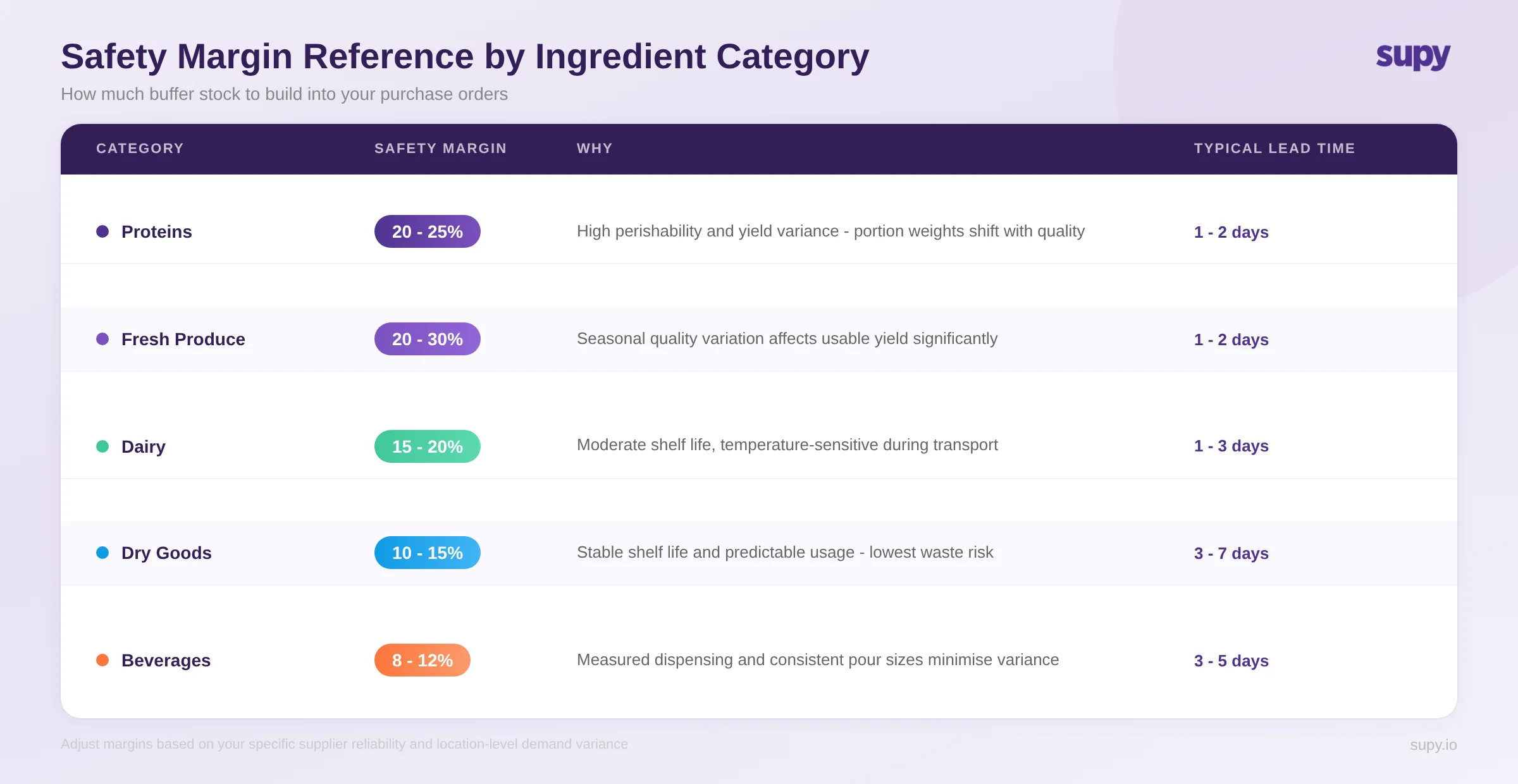
A few things worth stating clearly about these ranges. They are starting points, not fixed targets — your actual safety margins should be calibrated against your own supplier lead times and your own historical forecast error. Start here and refine over 90 days of live data. Multi-location operations should calculate safety margins per location, not as a group average. A central kitchen supplying satellite locations carries different lead time risk than a standalone restaurant ordering direct. And reduce safety margins on dry goods and ambient ingredients over time as your data quality improves — holding unnecessary buffer on items with a 90-day shelf life is dead working capital.

One pattern that consistently shows up across operators at the 10-plus location scale: over-ordering on perishables and under-ordering on ambient goods. The perishable over-ordering is visible (it creates waste), so it gets attention. The ambient under-ordering is invisible (it just means more frequent top-up orders at worse prices), so it does not. Safety margin calibration by category catches both.

Step 5: Connect Forecasts to Automated Purchasing

The final step is where forecasting converts from an analytical exercise into an operational workflow. A demand forecast that lives in a spreadsheet and requires manual translation into a purchase order is not a purchasing system — it is a reference document that may or may not get used consistently.

One finance director from a QSR group put it directly: "I very quickly nailed down the issue to the fact that we did not have a recipe costing system tied up to our POS system. I wish you were around by that time." The calculation existed. The link to purchasing did not.

Most manual forecasting processes break at the translation step — converting yield-adjusted ingredient demand into draft purchase orders. In a 10-location operation ordering from 15 suppliers twice a week, that manual translation alone is a 6 to 8 hour weekly task at minimum. Across operators using Supy's Predictive Orders module, teams reclaim an average of 40 hours per location per month previously spent on manual PO calculations and supplier communication.

In Supy, the connection between forecast and purchase order works like this: you choose your location, select a supplier, set the required delivery date, and specify the cover period — the number of days you want this order to sustain you. If your supplier delivers on Fridays and Tuesdays, you might set a five-day cover period for the Friday delivery. Supy then surfaces every ingredient you will need from that supplier across those five days — not every item in their catalogue, only the items your forecasted demand actually requires.

Each line shows your current on-hand quantity, your projected stock on the delivery date (accounting for consumption between now and then), and the calculated order quantity. Two benchmark columns run alongside: your most recent order quantity and your four-week ordering average. If the system suggests a quantity that deviates significantly from your typical pattern, the comparison flags it before you approve.

Supy's forecasting layer also ingests weather, public holidays, and local event data as inputs to the model, which meaningfully improves accuracy around peak demand periods that are predictable from an events calendar but invisible to a historical-data-only model. A sold-out concert venue two streets away on a Thursday evening is not in your POS history. It is in the events calendar. The distinction matters when you are ordering fresh proteins with two-day lead times.

Before any order reaches a supplier, your buyer reviews the draft, adjusts quantities where needed, and approves it. The forecast does the calculation; the buyer makes the final call.

The accuracy improvement compounds. As actual consumption is measured against forecasted demand, the model builds a feedback loop that tightens every subsequent forecast. Kokoro, a restaurant group using Supy across their estate, achieved a 28% reduction in ingredient wastage alongside 100% visibility into ingredient-level consumption across sites. The waste reduction was not the result of operational discipline changing — it was the result of the ordering process becoming accurate enough that over-ordering stopped being the default hedge against stock-outs.

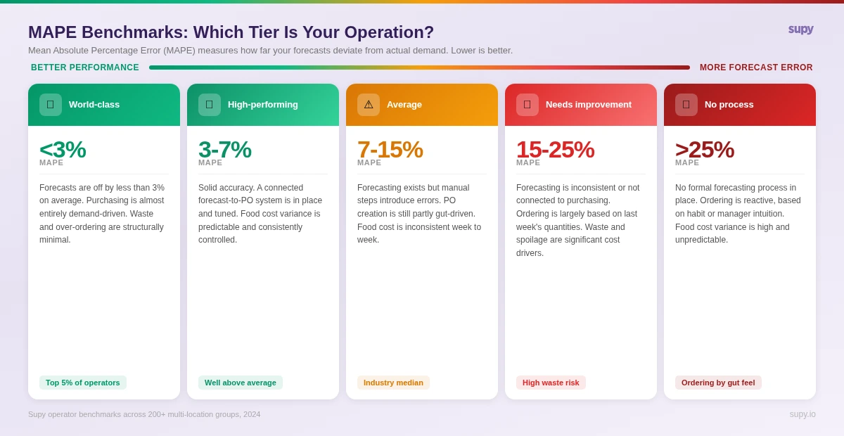
If your operation is sitting above 15% MAPE, the priority is data quality and basic process before methodology. Clean POS data, consistent recipe cards with yield factors, and a weekly review cadence will get you to the 7 to 15% band faster than any algorithm upgrade.

If you are already in the 7 to 15% range and looking to break through to 3 to 7%, the bottleneck is typically the manual calculation and transfer steps in your process, not the forecast model itself. The model is fine. The process around it is the problem.

Operators who set a hard accuracy target — one group on the platform targets 90% forecast accuracy as a KPI reviewed weekly — tend to improve faster than those who treat accuracy as a secondary metric. What gets measured gets managed. A forecast accuracy percentage sitting next to food cost on your weekly review report changes how seriously the team treats the data inputs.

About Supy

Supy is a back-of-house operations platform built for multi-location restaurant groups. The platform connects procurement, inventory management, and AI-powered demand forecasting into a single operational system — from POS-linked item-level sales forecasting through yield-adjusted ingredient demand calculation to Predictive Orders that generate draft purchase orders per supplier automatically. Teams using Supy's forecasting and purchasing modules typically achieve a 7% reduction in food costs and reclaim 40-plus hours per location per month previously spent on manual ordering processes.